Single-sample analysis • STID

Overview

This vignette presents a single-sample workflow in STID that starts from expanded niche metadata and systematically evaluates tissue composition, cell-type composition, spatial aggregation, colocalization, cell–cell communication, regulatory networks, and host–pathogen interactions within selected niches.

This vignette covers:

constructing a single-sample niche object from expanded niche metadata;
quantifying niche composition, aggregation, colocalization, and spatial gradients;
identifying niche-associated genes and enriched pathways;
inferring cell–cell communication, regulatory networks, and host-pathogen interaction.

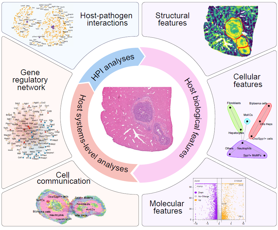
Overview of single-sample niche analysis.

Note: Before running the workflow, update the input STID object, niche metadata key, sample identifier, ROI columns, annotation columns, gene sets, reference database paths, pathogen gene prefix, plotting colors, and output group names to match the dataset under analysis.

Reference code: For more runnable code examples, please refer to the article code.

Prerequisites

library(tidyverse)
library(Seurat)
library(STID)

Note: The core workflow uses tidyverse, Seurat, and STID. Downstream sections additionally require resources such as CellChat, NicheNet, BLAST, ligand–receptor networks, and organism-specific STRING files. Prepare these dependencies before running the corresponding analyses.

Example data

This example uses the expanded focal-niche object generated by the infection-associated niche identification workflow. Here, STID_obj_expand contains expanded niche boundaries for the AE dataset, and the analysis focuses on the DPI_4_2 (PI4d) sample.

Note: Replace STID_obj_expand, M2_NicheExpand_AE_expand, DPI_4_2, batch, anno, and ROI-related columns with the corresponding object name, metadata keys, sample identifier, and annotation columns in your dataset.

niche_key <- "Niche"
expanded_niche_key <- "M2_NicheExpand_AE_expand"
example_sample_id <- "DPI_4_2"
celltype_column <- "anno"
sample_column <- "batch"

Add tissue-level annotations

Tissue-level annotations can be added before constructing the single-sample niche object. In this example, liver zonation is represented by nine periportal-to-pericentral layers and then collapsed into three broader zones.

Note: If tissue-level annotations are already available, skip this step and pass the existing metadata key to CreateSingleSampNiche().

geneset_list <- list(
  Pericentral = c(
    "Akr1c6", "Aldh1a1", "Car3", "Ces1c", "Cyp1a2", "Cyp2c37",
    "Cyp2c50", "Cyp2e1", "Gsta3", "Mgst1", "Mup11", "Mup17",
    "Mup18", "Oat", "Pon1", "Rgn"
  ),
  Periportal = c(
    "Alb", "Aldob", "Arg1", "Asl", "Cyp2f2", "Fbp1", "Hal",
    "Hpx", "Hsd17b13", "Mup20", "Pck1", "Slc25a47", "Trf", "Ass1"
  )
)

COLOR_DIS_CON <- STID::COLOR_DIS_CON

STID_obj_expand <- SpotDetect_Geneset(
  STID_obj_expand,
  geneset_list = geneset_list,
  score_method = "MeanExp",
  n_iter = 5,
  nbin = 24,
  seed = 10,
  PosThres_prob = 0,
  PosThres_score = 0,
  pt_size = 0.25,
  col = COLOR_DIS_CON,
  black_bg = FALSE,
  blur_method = NULL,
  plot_method = "single",
  grp_nm = "AE_detect_geneset_stratify"
)

expanded_meta <- GetMetaData(
  STID_obj_expand,
  meta_key = "M2_SpotDetect_Geneset_AE_detect_geneset_stratify",
  add_coord = TRUE
)[[1]]

expanded_meta <- expanded_meta %>%
  rownames_to_column(var = "cell_id") %>%
  group_by(.data[[sample_column]]) %>%
  mutate(PV_CV = Periportal - Pericentral) %>%
  mutate(label = cut_number(PV_CV, n = 9, labels = FALSE)) %>%
  mutate(label9 = paste0("Layer_", as.numeric(label))) %>%
  mutate(
    label3 = case_when(
      label9 %in% c("Layer_1", "Layer_2", "Layer_3") ~ "Pericentral",
      label9 %in% c("Layer_4", "Layer_5", "Layer_6") ~ "Midzone",
      TRUE ~ "Periportal"
    ),
    label3 = factor(label3, levels = c("Pericentral", "Midzone", "Periportal")),
    merge_label = if_else(ROI_region == "edge", "edge", label9, missing = label9)
  ) %>%
  ungroup() %>%
  column_to_rownames(var = "cell_id")

STID_obj_expand <- AddMetaData(
  STID_obj = STID_obj_expand,
  meta_key = "hep_layer9",
  add_data = expanded_meta
)

LAYER_COLORS <- c(
  "red",
  rev(c(
    "#440154FF", "#472D7BFF", "#3B528BFF", "#2C728EFF", "#21908CFF",
    "#27AD81FF", "#5DC863FF", "#AADC32FF", "#FDE725FF"
  ))
)

Plot_Spatial(
  plot_data = expanded_meta,
  x_colnm = "x",
  y_colnm = "y",
  group_by = "merge_label",
  facet_grpnm = sample_column,
  datatype = "discrete",
  col = list(dis = LAYER_COLORS, con = NULL),
  pt_size = 1.1,
  vmin = NULL,
  vmax = "p99",
  title = NULL,
  subtitle = NULL,
  black_bg = FALSE
)

Construct a single-sample niche object

CreateSingleSampNiche() organizes niche, edge, center, and bystander-region metadata for downstream analyses. AddSSNicheCells() then adds selected cell-level or tissue-level labels to the single-sample niche object.

Note: Update meta_key, ROI_type, pos_colnm, center_colnm, edge_colnm, all_label_colnm, all_dist_colnm, and other_colnm to match the metadata generated in the niche identification workflow.

STID_obj_SS <- CreateSingleSampNiche(
  STID_obj = STID_obj_expand,
  niche_key = niche_key,
  meta_key = list(c(expanded_niche_key, "hep_layer9")),
  ROI_type = "ROI",
  pos_colnm = "ROI_label",
  center_colnm = "ROI_center",
  edge_colnm = "ROI_edge",
  all_label_colnm = "All_ROI_label",
  all_dist_colnm = "All_Dist2ROIcenter",
  other_colnm = "label9",
  description = NULL
)

STID_obj_SS <- AddSSNicheCells(
  STID_obj = STID_obj_SS,
  meta_key = "hep_layer9",
  select_colnm = "label3",
  niche_key = niche_key
)

Quantify tissue and cell-type composition

CalSampComp() summarizes the relative abundance of tissue layers or cell types across niches. Apply the same function to different annotation systems by changing group_by.

Note: Update group_by and loop_id according to the annotation columns and sample identifiers in your dataset.

col_lasso <- c(
  "HsPCs" = "#E41A1C",
  "Hepatocytes" = "grey95",
  "Infla Heps" = "#4DAF4A",
  "Fibroblasts" = "#984EA3",
  "Cho/Spp1+ cells" = "#FFFF33",
  "Spp1+ MoMFs" = "#FF7F00",
  "MoKCs" = "#377EB8",
  "Neutrophils" = "#F781BF",
  "B/plasma cells" = "#A65628",
  "Others" = "#8DA0CB"
)
col_lasso2 <- c(
  "HsPCs" = "#E41A1C",
  "Hepatocytes" = "#66C2A5",
  "Infla Heps" = "#4DAF4A",
  "Fibroblasts" = "#984EA3",
  "Cho/Spp1+ cells" = "#FFFF33",
  "Spp1+ MoMFs" = "#FF7F00",
  "MoKCs" = "#377EB8",
  "Neutrophils" = "#F781BF",
  "B/plasma cells" = "#A65628",
  "Others" = "#8DA0CB"
)

# Tissue-layer composition
CalSampComp(
  STID_obj = STID_obj_SS,
  niche_key = niche_key,
  group_by = "label9",
  loop_id = "LoopAllSamp",
  col = rev(c(
    "#440154FF", "#472D7BFF", "#3B528BFF", "#2C728EFF", "#21908CFF",
    "#27AD81FF", "#5DC863FF", "#AADC32FF", "#FDE725FF"
  )),
  return_data = FALSE
)

# Cell-type composition
CalSampComp(
  STID_obj = STID_obj_SS,
  niche_key = niche_key,
  group_by = celltype_column,
  loop_id = "LoopAllSamp",
  col = col_lasso,
  return_data = FALSE
)

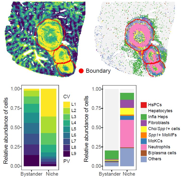
Tissue-layer and cell-type composition within single-sample niches.

Cell aggregation index

CalSampCAI() measures whether cells of the same type form local aggregates within niches. The analysis uses nearest-neighbor distances among same-type cells and summarizes both regional aggregation scores and the fraction of cells located in connected aggregates.

Note: Set k_neighbors according to spatial geometry and resolution. Square-grid data commonly use eight neighbors, whereas hex-grid data commonly use six. Update min_agg_size, dist_thres, group_by, and loop_id according to the expected aggregate size.

cell_aggregation <- CalSampCAI(
  STID_obj = STID_obj_SS,
  niche_key = niche_key,
  group_by = celltype_column,
  loop_id = "LoopAllSamp",
  k_neighbors = 8,
  min_agg_size = 10,
  dist_thres = 1,
  col = col_lasso
)

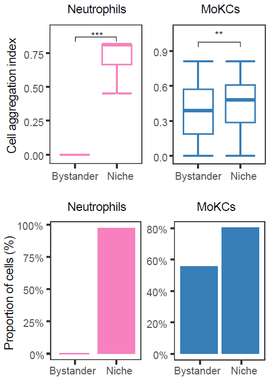
Cell aggregation within single-sample niches.

Colocalization analysis

CalSampCoLoc() evaluates spatial colocalization between cell types or gene-expression features. Proximity-based analysis summarizes neighborhood enrichment, whereas expression-based analysis estimates whether neighboring features improve prediction of a target feature.

Note: Update group_by, loop_id, method, and mistyR_params according to the feature type, sample identifier, and spatial scale of interest. The squidpy option requires a Python environment accessible through reticulate.

# mistyR
cell_colocalization_mistyR <- CalSampCoLoc(
  STID_obj = STID_obj_SS,
  niche_key = niche_key,
  group_by = celltype_column,
  loop_id = example_sample_id,
  method = "mistyR",
  mistyR_params = c(15, 10),
  return_data = TRUE
)

# squidpy
cell_colocalization_squidpy <- CalSampCoLoc(
  STID_obj = STID_obj_SS,
  niche_key = niche_key,
  group_by = celltype_column,
  loop_id = example_sample_id,
  method = "squidpy",
  mistyR_params = c(15, 10),
  return_data = TRUE
)

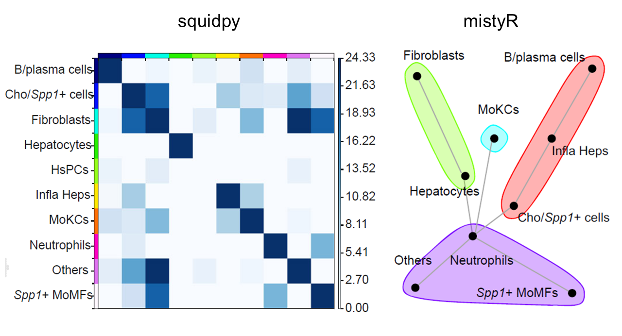
Spatial colocalization analysis within single-sample niches.

Selected cell-type or gene-pair colocalization patterns can be displayed directly in spatial coordinates.

Note: Replace group_use, features, and loop_id with cell-type or gene pairs relevant to the biological question.

# Cell-type pair
Plot_SpatialCoLoc(
  STID_obj = STID_obj_SS,
  niche_key = niche_key,
  group_by = celltype_column,
  group_use = c("Neutrophils", "Spp1+ MoMFs"),
  loop_id = "LoopAllSamp"
)

# Gene pair
Plot_SpatialCoLoc(
  STID_obj = STID_obj_SS,
  niche_key = niche_key,
  group_by = NULL,
  group_use = NULL,
  features = c("Ccl3", "Ccr1"),
  loop_id = "LoopAllSamp"
)

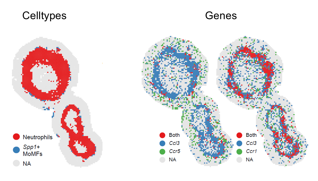
Spatial visualization of selected colocalized cell types or genes.

Cell composition gradient analysis

Plot_DistLine_Ratio() summarizes how cell-type proportions change with distance from niche centers. Cells are binned along the niche-to-bystander axis, and fitted trends are used to visualize composition shifts across niche boundaries.

Note: Update celltypes, group_by, loop_id, facet_grpnm, meta_key, and coord_interval_ratio according to the cell annotations, sample identifier, metadata key, and spatial scale used in your analysis.

Plot_DistLine_Ratio(
  STID_obj = STID_obj_SS,
  celltypes = c(
    "Hepatocytes", "Spp1+ MoMFs", "Neutrophils",
    "Fibroblasts", "Cho/Spp1+ cells"
  ),
  group_by = celltype_column,
  loop_id = example_sample_id,
  facet_grpnm = sample_column,
  meta_key = expanded_niche_key,
  coord_interval_ratio = 8
)

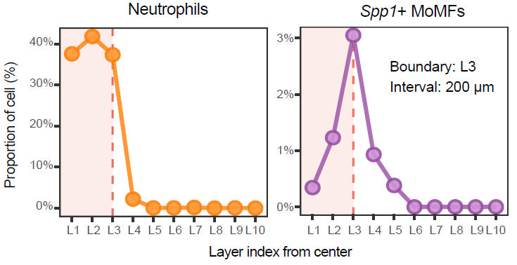
Distance-dependent niche-associated gradients.

Differential gene expression analysis

CalSampDEGs() identifies genes associated with niches globally or within selected cell types. This example compares niche and bystander regions using Seurat::FindAllMarkers() with adjusted p-value and log fold-change thresholds. The resulting gene sets can be used for downstream functional enrichment and regulatory network analyses.

Note: Update assay_id, layer_id, group_by, group_value, filtering thresholds, and remove_genes according to the input object, species, and analysis objective.

SS_DEGs <- CalSampDEGs(
  STID_obj = STID_obj_SS,
  niche_key = niche_key,
  assay_id = "Spatial",
  layer_id = "counts",
  loop_id = "LoopAllSamp",
  padj_thres = 0.05,
  logfc_thres = 1,
  adjust_method = "BH",
  col = col_lasso2,
  group_by = celltype_column,
  group_value = c("Infla Heps", "Fibroblasts", "Neutrophils", "MoKCs"),
  remove_genes = grep("^Gm", rownames(STID_obj_SS), value = TRUE)
)

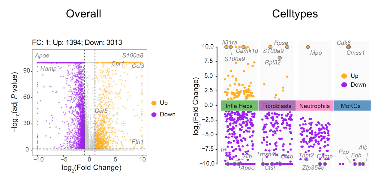
Differentially expressed genes associated with single-sample niches.

Gene set enrichment analysis

GeneEnrichment() tests functional enrichment using differential genes or user-supplied up- and down-regulated gene sets. This example performs Gene Ontology and KEGG over-representation analysis.

Note: Replace up_gene and down_gene with genes derived from the differential expression results. Update method, go_ont, and organism-specific annotation settings to match the species and database used in your analysis.

up_gene <- SS_DEGs$DPI_4_2$data$Overall_DEGs$gene[SS_DEGs$DPI_4_2$data$Overall_DEGs$change == "Up"]
down_gene <- SS_DEGs$DPI_4_2$data$Overall_DEGs$gene[SS_DEGs$DPI_4_2$data$Overall_DEGs$change == "Down"]
enrichment_results <- GeneEnrichment(
  STID_obj = STID_obj_SS,
  DEGs = NULL,
  up_gene = up_gene,
  down_gene = down_gene,
  method = "GO_KEGG",
  go_ont = "BP",
  return_data = TRUE
)

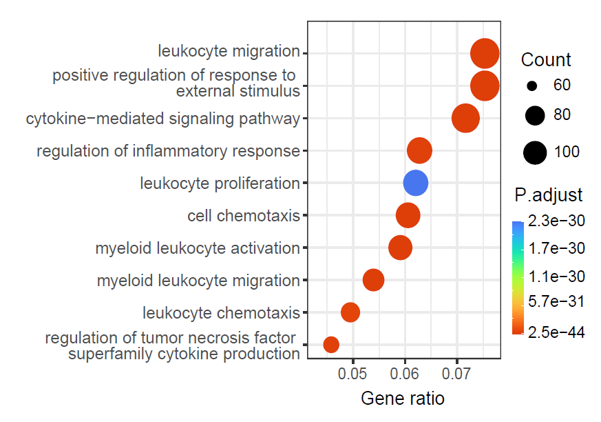
Functional enrichment of niche-associated genes.

Cell–cell communication analysis

CalSampCellComm() integrates ligand–receptor expression with spatial constraints to infer niche-associated communication. The output summarizes signaling pathways, sender and receiver cell types, and ligand–receptor pairs within niches.

Note: Update group_by, assay_id, layer_id, loop_id, interaction.range, spatial scaling parameters, and output directory according to the spatial platform, bin size, and communication model.

cell_communication <- CalSampCellComm(
  STID_obj = STID_obj_SS,
  niche_key = niche_key,
  group_by = NULL,
  assay_id = "Spatial",
  layer_id = "counts",
  loop_id = "LoopAllSamp",
  col = col_lasso2,
  is_Spatial = TRUE,
  spatial.factors = NULL,
  interaction.range = 250,
  return_data = TRUE,
  grp_nm = "CalSampCellComm",
  dir_nm = "M3_CalSampCellComm"
)

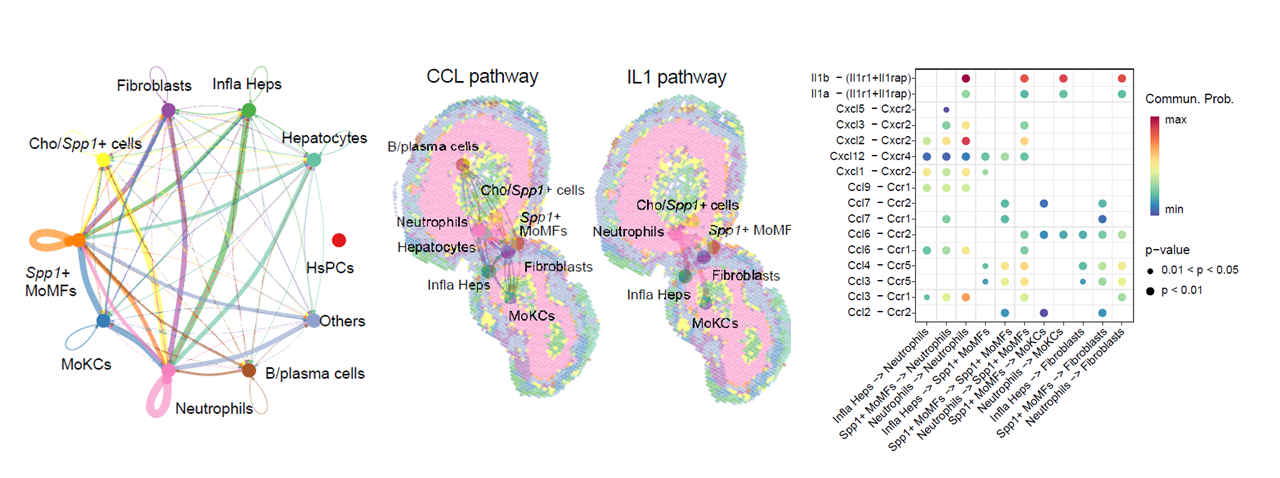
Cell-cell communication within single-sample niches.

Gene regulatory network analysis

CalSampGRN() prioritizes candidate ligands and downstream target genes using ligand–receptor and ligand-target priors. This analysis links sender-cell ligands to receiver-cell regulatory programs in the niche microenvironment.

Note: Update NicheNet reference paths, species-specific reference files, sender and receiver cell types, target_features, expression thresholds, top-ligand and top-target settings, and loop_id. The reference matrices and networks used in this section are not generated by STID; download the appropriate species-specific files from the official NicheNet resource, store them locally, and update the paths below. Retaining local copies and recording their versions improves reproducibility.

# Load NicheNet reference data downloaded from the official resource
ligand_target_matrix <- readRDS(
  "./inputdata/Demo/CalSampGRN/NicheNet_V2/ligand_target_matrix_nsga2r_final_mouse.rds"
)
lr_network <- readRDS(
  "./inputdata/Demo/CalSampGRN/NicheNet_V2/lr_network_mouse_21122021.rds"
)
weighted_networks <- readRDS(
  "./inputdata/Demo/CalSampGRN/NicheNet_V2/weighted_networks_nsga2r_final_mouse.rds"
)
gr_network <- readRDS(
  "./inputdata/Demo/CalSampGRN/NicheNet_V2/gr_network_mouse_21122021.rds"
)
sig_networks <- readRDS(
  "./inputdata/Demo/CalSampGRN/NicheNet_V2/signaling_network_mouse_21122021.rds"
)
ligand_tf_matrix <- readRDS(
  "./inputdata/Demo/CalSampGRN/NicheNet_V2/ligand_tf_matrix_nsga2r_final_mouse.rds"
)

ref_data <- list(
  ligand_target_matrix = ligand_target_matrix,
  lr_network = lr_network,
  weighted_networks = weighted_networks,
  gr_network = gr_network,
  sig_networks = sig_networks,
  ligand_tf_matrix = ligand_tf_matrix
)

DEGs_gene <- SS_DEGs$DPI_4_2$data$Overall_DEGs %>%
  filter(avg_log2FC > 1, p_val_adj < 0.05) %>%
  pull(gene) %>%
  unique()

# Infer ligand-driven regulatory networks within the niche
regulatory_network <- CalSampGRN(
  STID_obj = STID_obj_SS,
  niche_key = niche_key,
  group_by = NULL,
  ref_data = ref_data,
  sender_celltypes = c("Infla Heps", "Neutrophils", "Spp1+ MoMFs"),
  receiver_celltypes = c("Neutrophils", "Spp1+ MoMFs", "MoKCs", "Fibroblasts"),
  target_features = DEGs_gene,
  expression_pct = 0.1,
  top_ligand_num = 10,
  top_target_num = 10,
  loop_id = example_sample_id,
  return_data = TRUE
)

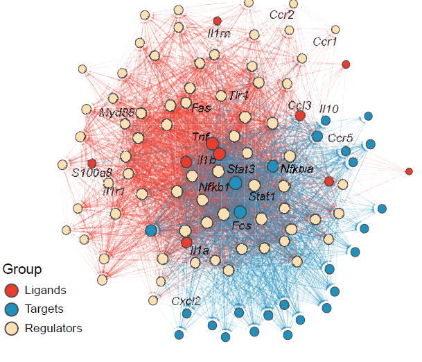
Ligand-driven regulatory networks within single-sample niches.

Host–pathogen interaction analysis

This section evaluates host-pathogen relationships at gene and protein levels. Gene-level analysis identifies host genes spatially correlated with pathogen gene abundance, whereas protein-level analysis prioritizes candidate associations supported by sequence similarity and host protein-interaction networks.

Host-pathogen gene correlation

CalSampGeneCor() quantifies correlations between pathogen-derived genes and host genes within selected niches. This analysis prioritizes host genes whose spatial expression is associated with pathogen burden.

Note: Update the pathogen gene prefix in pattern, top-pathogen-gene number, host target genes, feature column names, correlation method, assay and layer names, and loop_id according to the dataset and pathogen annotation scheme.

high_exp_pathogen_genes <- GetTopGenes(
  STID_obj_SS,
  top_n = 7,
  pattern = "EmuJ-",
  grp_by_samp = FALSE,
  grp_by_celltype = FALSE,
  assay_id = "Spatial",
  layer_id = "counts"
)

DEGs_gene <- SS_DEGs$DPI_4_2$data$Overall_DEGs %>%
  filter(avg_log2FC > 1, p_val_adj < 0.05) %>%
  pull(gene) %>%
  unique()

gene_correlations <- CalSampGeneCor(
  STID_obj = STID_obj_SS,
  loop_id = example_sample_id,
  niche_key = niche_key,
  p.features = high_exp_pathogen_genes,
  h.features = DEGs_gene,
  p.feature_colnm = "all_gene_nCount(sum)",
  method = "spearman",
  assay_id = "Spatial",
  layer_id = "counts",
  return_data = TRUE
)

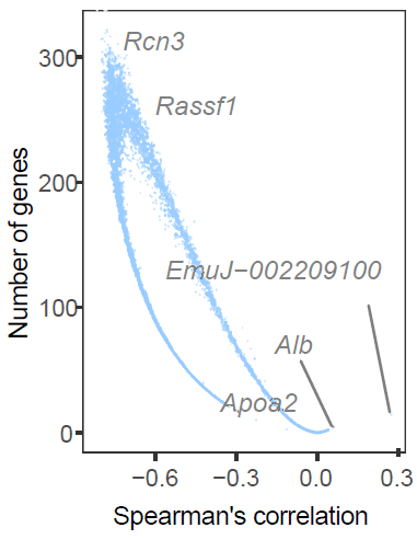
Host-pathogen gene associations within single-sample niches.

Host-pathogen protein association

CalSampPPI() integrates pathogen and host protein FASTA files, symbol-to-protein mappings, BLAST alignment, and STRING networks to infer candidate host-pathogen protein associations.

Note: Update FASTA files, symbol-to-protein mapping files, BLAST parameters, STRING version, score thresholds, pathogen features, and host features according to the organisms, protein identifiers, and confidence criteria used in your analysis. The pathogen and host FASTA files, symbol-to-protein mappings, BLAST resources, and STRING network data must be obtained from the corresponding official databases or project websites before this analysis. Store the files locally, verify that their identifiers are mutually compatible, and update all paths and version parameters below.

# Prepare officially sourced input files and analysis parameters
pathogen_fasta_path <- "./inputdata/Demo/CalSampPPI/EmuJ_protein.fa"
pathogen_symbol2protein_path <- "./inputdata/Demo/CalSampPPI/EmuJ_symbol2protein.txt"
host_fasta_path <- "./inputdata/Demo/CalSampPPI/mouse_protein.fa"
host_symbol2protein_path <- "./inputdata/Demo/CalSampPPI/mouse_symbol2protein.txt"

DEGs_gene <- SS_DEGs$DPI_4_2$data$Overall_DEGs %>%
  filter(avg_log2FC > 1, p_val_adj < 0.05) %>%
  pull(gene) %>%
  unique()

# Infer host-pathogen protein associations using sequence similarity and STRING interactions
protein_associations <- CalSampPPI(
  STID_obj = STID_obj_SS,
  p.fasta_path = pathogen_fasta_path,
  h.fasta_path = host_fasta_path,
  p.symbol2protein_path = pathogen_symbol2protein_path,
  h.symbol2protein_path = host_symbol2protein_path,
  p.features = high_exp_pathogen_genes,
  h.features = DEGs_gene,
  BLAST_tool = "blastp",
  dbtype = "prot",
  BLAST_args = "-evalue 1e-10 -max_target_seqs 5 -max_hsps 50 -num_threads 4",
  BLAST_fil_args = "pident > 40, evalue < 1e-10, bitscore > 100, length > 100",
  version_STRING = "12.0",
  score_thre_only = 100,
  score_thre_all = 800
)

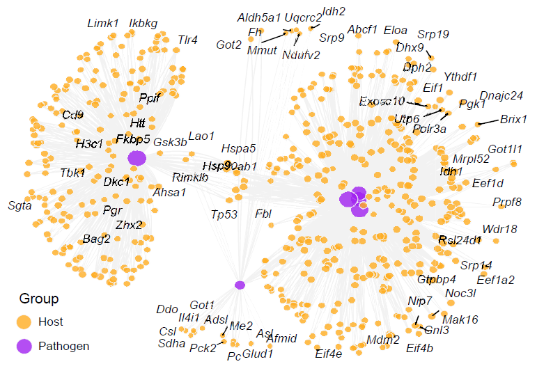
Host-pathogen protein association network inferred from sequence similarity and STRING interactions.

Notes

Confirm that ROI labels, center labels, edge labels, distance columns, tissue-layer labels, and cell-type annotations are present before downstream analysis.
Select neighborhood size, distance thresholds, and bin numbers according to spatial resolution and expected niche size.
Use dataset-specific gene sets, cell types, ligand–receptor references, and host-pathogen protein resources.

Next steps

This vignette characterized infection-associated niches within individual samples, including niche composition, spatial organization, molecular programs, cell–cell communication, gene regulatory networks, and host–pathogen interactions. In the next vignette, we will extend these analyses to multiple samples to compare niche features across conditions or model temporal niche dynamics during infection progression.

Session information

sessionInfo()
#> R version 4.2.0 (2022-04-22 ucrt)
#> Platform: x86_64-w64-mingw32/x64 (64-bit)
#> Running under: Windows 10 x64 (build 22000)
#> 
#> Matrix products: default
#> 
#> locale:
#> [1] LC_COLLATE=Chinese (Simplified)_China.utf8 
#> [2] LC_CTYPE=Chinese (Simplified)_China.utf8   
#> [3] LC_MONETARY=Chinese (Simplified)_China.utf8
#> [4] LC_NUMERIC=C                               
#> [5] LC_TIME=Chinese (Simplified)_China.utf8    
#> 
#> attached base packages:
#> [1] stats     graphics  grDevices utils     datasets  methods   base     
#> 
#> loaded via a namespace (and not attached):
#>  [1] digest_0.6.35     R6_2.6.1          jsonlite_1.8.8    lifecycle_1.0.5  
#>  [5] evaluate_1.0.1    cachem_1.1.0      rlang_1.1.7       cli_3.6.5        
#>  [9] rstudioapi_0.15.0 fs_1.6.3          jquerylib_0.1.4   bslib_0.8.0      
#> [13] ragg_1.3.0        rmarkdown_2.29    pkgdown_2.2.0     textshaping_0.3.6
#> [17] desc_1.4.3        tools_4.2.0       htmlwidgets_1.6.4 yaml_2.3.10      
#> [21] xfun_0.49         fastmap_1.2.0     compiler_4.2.0    systemfonts_1.0.4
#> [25] htmltools_0.5.8.1 knitr_1.49        sass_0.4.9