Pathogen background correction • STID

Overview

This vignette describes how to perform pathogen background correction for spatial transcriptomic data of infectious diseases using STID.

Accurate detection of pathogen-derived background signals requires explicit modeling of background contamination. In STID, background correction uses reference background or control samples to estimate the distribution of pathogen-associated features and reduce spurious signals before downstream spatial transcriptomic analysis of infectious diseases.

This vignette covers:

preparing a processed STID object and a pathogen feature list;
selecting background or control samples for background modeling;
running CorrectBackground();
summarizing pathogen-derived background signal before and after correction;
generating spatial distribution maps of pathogen-derived background signals.

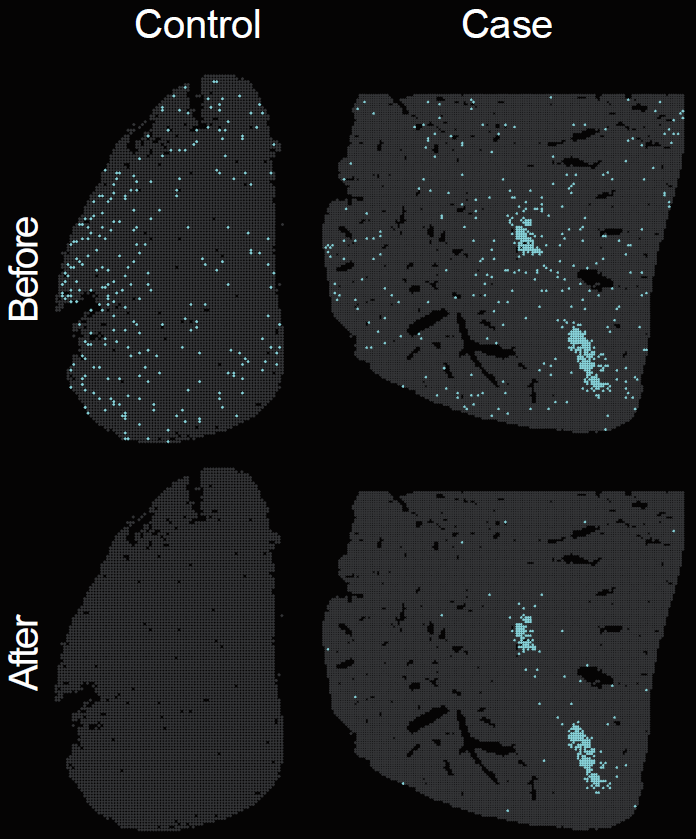
Spatial distribution of pathogen-derived background signal before and after background correction.

Note: Update the STID object name, pathogen feature list, background sample IDs, assay name, layer name, pathogen gene prefix, group names, and output directory according to the dataset used in your analysis.

Reference code: For more runnable code examples, please refer to the article code.

Prerequisites

library(tidyverse)
library(Seurat)
library(STID)

Example data

This vignette uses the processed AE STID_obj object and a pathogen feature list that have already been generated in the preprocessing step.

Note: Replace STID_obj, pathogen_genes, and DPI_0_1 with the object name, pathogen feature vector, and background or control sample IDs used in your dataset.

STID_obj_before <- STID_obj

# Update this vector to match the background or control samples in your dataset.
background_sample_ids <- c("DPI_0_1")

# Update this object if your pathogen feature list uses a different name.
background_features <- pathogen_genes

Background correction

To reduce background noise from pathogen-associated genes, a control-based background correction strategy is applied. For each pathogen-associated feature, the 95th percentile of nonzero expression values in the background samples is calculated and used as the background expression threshold.

To account for differences in sequencing depth, this threshold is adjusted by the ratio of average unique molecular identifier (UMI) counts between the background samples and all samples. The adjusted threshold is then subtracted from expression values across all spots or cells, and negative corrected values are set to zero.

options("parallel_workers" = 4)

STID_obj_after <- CorrectBackground(
  STID_obj = STID_obj_before,
  bg_samp_id = background_sample_ids,
  bg_features = background_features,
  PosThres_prob = 0.95,
  assay_id = "Spatial",
  layer_id = "counts",
  grp_nm = "Final_CE_0.95",
  dir_nm = "M1_CorrectBackground"
)

The choice of PosThres_prob determines the balance between sensitivity and specificity. It should be calibrated according to sequencing depth, background signal level, and expected pathogen load.

The following figure summarizes pathogen-derived background signal after background correction.

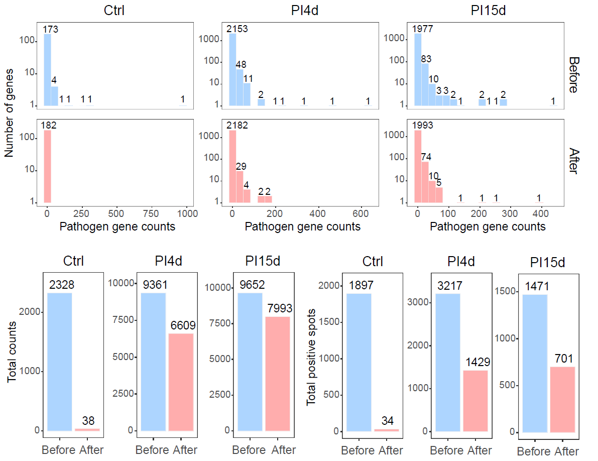
Summary of pathogen-derived background signal after background correction.

Spatial distribution of pathogen-derived background signal

This section generates exploratory spatial maps of pathogen-derived background signal before and after background correction. Formal detection of infection-associated positive spots is described in the Infection associated spot detection vignette.

Note: Update the pathogen gene prefix in pattern, the pathogen feature vector, metadata key, assay name, layer name, and output group names according to your dataset.

Calculate the overall expression of pathogen genes and add the results to meta.data.

high_exp_genes <- GetTopGenes(
  STID_obj_before,
  top_n = 10,
  pattern = "EmuJ-",
  grp_by_samp = FALSE,
  grp_by_celltype = FALSE,
  assay_id = "Spatial",
  layer_id = "counts"
)

# before correction
raw_pathogen_signal_before <- GetGeneStat(
  STID_obj = STID_obj_before,
  features = pathogen_genes,
  prefix = "all_gene",
  func = "sum"
)

STID_obj_before <- AddMetaColumn(
  STID_obj = STID_obj_before,
  add_data = raw_pathogen_signal_before,
  meta_key = "raw",
  ignore_rownm = FALSE
)

# after correction
raw_pathogen_signal_after <- GetGeneStat(
  STID_obj = STID_obj_after,
  features = pathogen_genes,
  prefix = "all_gene",
  func = "sum"
)

STID_obj_after <- AddMetaColumn(
  STID_obj = STID_obj_after,
  add_data = raw_pathogen_signal_after,
  meta_key = "raw",
  ignore_rownm = FALSE
)

Using identical parameters, calculate the spatial distribution of pathogen-infected positive spots in the STID object before and after pathogen background correction.

# before correction
pathogen_signal_columns_before <- grep(
  "all_gene",
  colnames(STID_obj_before@meta.data),
  value = TRUE
)

STID_obj_before <- SpotDetect_Gene(
  STID_obj_before,
  features = high_exp_genes,
  feature_colnm = pathogen_signal_columns_before,
  PosThres_prob = 0,
  PosThres_count = 1,
  col = c("grey20", "#80FFFF"),
  black_bg = TRUE,
  pt_size = 1,
  blur_method = NULL,
  blur_n = 1,
  blur_sigma = 0.5,
  plot_method = "single",
  grp_nm = "CE_correct_before_all_gene_black"
)

# after correction
pathogen_signal_columns_after <- grep(
  "all_gene",
  colnames(STID_obj_after@meta.data),
  value = TRUE
)

STID_obj_after <- SpotDetect_Gene(
  STID_obj_after,
  features = high_exp_genes,
  feature_colnm = pathogen_signal_columns_after,
  PosThres_prob = 0,
  PosThres_count = 1,
  col = c("grey20", "#80FFFF"),
  black_bg = TRUE,
  pt_size = 1,
  blur_method = NULL,
  blur_n = 1,
  blur_sigma = 0.5,
  plot_method = "single",
  grp_nm = "CE_correct_after_all_gene_black"
)

The following figure shows the spatial distribution of pathogen-derived background signal before and after background correction.

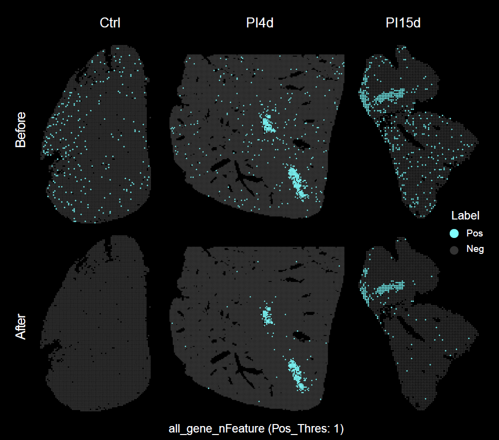
Spatial distribution of pathogen-derived background signal before and after background correction.

Notes

Apply pathogen background correction before downstream infection-associated spatial transcriptomic analysis.
Confirm that background samples represent true baseline conditions before running correction.
The corrected STID object preserves the original object structure while updating pathogen gene expression.
Recalibrate PosThres_prob when applying this workflow to datasets with different sequencing depth, pathogen burden, or background contamination levels.

Next steps

This vignette generated a background-corrected STID object and reduced nonspecific pathogen-derived signals in control or background samples. In the next vignette, we will use the corrected expression matrix to identify pathogen-infected spots and host-responsive spots based on gene expression or gene set scores.

Session information

sessionInfo()
#> R version 4.2.0 (2022-04-22 ucrt)
#> Platform: x86_64-w64-mingw32/x64 (64-bit)
#> Running under: Windows 10 x64 (build 22000)
#> 
#> Matrix products: default
#> 
#> locale:
#> [1] LC_COLLATE=Chinese (Simplified)_China.utf8 
#> [2] LC_CTYPE=Chinese (Simplified)_China.utf8   
#> [3] LC_MONETARY=Chinese (Simplified)_China.utf8
#> [4] LC_NUMERIC=C                               
#> [5] LC_TIME=Chinese (Simplified)_China.utf8    
#> 
#> attached base packages:
#> [1] stats     graphics  grDevices utils     datasets  methods   base     
#> 
#> loaded via a namespace (and not attached):
#>  [1] digest_0.6.35     R6_2.6.1          jsonlite_1.8.8    lifecycle_1.0.5  
#>  [5] evaluate_1.0.1    cachem_1.1.0      rlang_1.1.7       cli_3.6.5        
#>  [9] rstudioapi_0.15.0 fs_1.6.3          jquerylib_0.1.4   bslib_0.8.0      
#> [13] ragg_1.3.0        rmarkdown_2.29    pkgdown_2.2.0     textshaping_0.3.6
#> [17] desc_1.4.3        tools_4.2.0       htmlwidgets_1.6.4 yaml_2.3.10      
#> [21] xfun_0.49         fastmap_1.2.0     compiler_4.2.0    systemfonts_1.0.4
#> [25] htmltools_0.5.8.1 knitr_1.49        sass_0.4.9